Advanced Example

In this example we illustrate the use of PHRINGE with manually created Observation, Instrument, and Scene objects. In addition, we show how to access additional information that is generated during the simulation.

We will again create synthetic data for the observation of an Earth twin araound a Sun twin at 10 pc.

Import the Required Modules

import astropy.units as u
import matplotlib.pyplot as plt
import torch

from phringe.core.instrument import Instrument
from phringe.core.observation import Observation
from phringe.core.perturbations.power_law_psd_perturbation import PowerLawPSDPerturbation
from phringe.core.scene import Scene
from phringe.core.sources.exozodi import Exozodi
from phringe.core.sources.local_zodi import LocalZodi
from phringe.core.sources.planet import Planet
from phringe.core.sources.star import Star
from phringe.lib.array_configuration import XArrayConfiguration
from phringe.lib.baseline import OptimalNullingBaseline
from phringe.lib.beam_combiner import DoubleBracewell
from phringe.main import PHRINGE

Setup PHRINGE

Create the Main PHRINGE Object

PHRINGE is optimized to run on GPUs, but can also be run on CPUs. This can be specified using the device argument and relies on torch. For reproducibility, seed can be set to a specific value, resulting in identical results for each run. Note that seed=None results in the use of a random seed each run. The grid_size parameter specifies the number of grid points in the spatial domain. The larger the grid size, the more accurate the results, but the longer the computation time.

phringe = PHRINGE(device=torch.device('cuda:1'), seed=42, grid_size=60)

Create and Set an Observation

Arguments that require numerical values with units can be passed either as 1. astropy quantities, e.g. 10 * u.m 2. strings with units, e.g. '10 m', or 3. floats (ints), assuming SI units, e.g. 10.

The use of astropy quantities is recommended for clarity.

obs = Observation(
    solar_ecliptic_latitude=0 * u.deg,  # Alternatively: '0 deg' or 0
    total_integration_time=1 * u.day,  # Alternatively: '1 d' or 86400
    detector_integration_time=600 * u.s,  # Alternatively: '600 s' or 600
    modulation_period=1 * u.day,  # Alternatively: '1 d' or 86400
    nulling_baseline=OptimalNullingBaseline(  # Alternatively a fixed value, e.g. 10 * u.m
        angular_star_separation=0.1 * u.arcsec,
        wavelength=10 * u.um,
        sep_at_max_mod_eff=DoubleBracewell.sep_at_max_mod_eff[0]
    ),
    # host_star_radius=1 * u.Rsun,  # Only required as a reference if no star is present in the scene
    # host_star_temperature=5780 * u.K,  # Only required as a reference if no star is present in the scene
    # host_star_mass=1*u.Msun,  # Only required as a reference if no star is present in the scene
    # host_star_distance=10 * u.pc,  # Only required as a reference if no star is present in the scene
    # host_star_right_ascension=10 * u.hourangle,  # Only required as a reference if no star is present in the scene
    # host_star_declination=45 * u.deg,  # Only required as a reference if no star is present in the scene
)
phringe.set(obs)

Note: After initialization, the class attributes are converted to SI units and stored as floats, as astropy quantiteis can have a significant impact on performance. Consider, for instance, the total integration time, which has been converted to a float in seconds:

obs.total_integration_time

np.float64(86400.0)

Create and Set an Instrument

An instrument can be created manually using the Instrument class (see here for the class documentation) or by using a predefined instrument from the library. Here, we use the predefined LIFE baseline architecture as our instrument.

inst = Instrument(
    array_configuration_matrix=XArrayConfiguration.acm,
    complex_amplitude_transfer_matrix=DoubleBracewell.catm,
    kernels=DoubleBracewell.kernels,
    aperture_diameter=3 * u.m,
    nulling_baseline_min=8 * u.m,
    nulling_baseline_max=100 * u.m,
    throughput=0.12,
    quantum_efficiency=0.7,
    spectral_resolving_power=20,
    wavelength_min=4 * u.um,
    wavelength_max=18.5 * u.um,
    wavelength_bands_boundaries=[],  # Alternatively e.g. ['9 um']
    amplitude_perturbation=PowerLawPSDPerturbation(coefficient=1, rms=0.1 * u.percent),
    phase_perturbation=PowerLawPSDPerturbation(coefficient=1, rms=1.5 * u.nm, chromatic=True),
    polarization_perturbation=PowerLawPSDPerturbation(coefficient=1, rms=0.001 * u.rad)
)
phringe.set(inst)

Note: Attributes of objects can also be updated. For instance, changing the aperture diameter from the predefined value to 3.5 m:

print(f'Predefined aperture diameter: {inst.aperture_diameter}')

inst.aperture_diameter = 3.5  # Attributes are stored as floats (see above), so we input floats in SI units

print(f'Updated aperture diameter: {inst.aperture_diameter}')

Predefined aperture diameter: 3.0
Updated aperture diameter: 3.5

For the instrument we have defined we can now e.g. check the resulting wavelength bins. This depends on its minimum and maximum wavelengths and spectral resolving power:

phringe.get_wavelength_bin_centers()
phringe.get_wavelength_bin_centers().cpu().numpy()  # as a numpy array

array([4.10256416e-06, 4.31295211e-06, 4.53412895e-06, 4.76664854e-06,
       5.01109207e-06, 5.26807116e-06, 5.53822838e-06, 5.82224038e-06,
       6.12081658e-06, 6.43470457e-06, 6.76468972e-06, 7.11159691e-06,
       7.47629383e-06, 7.85969405e-06, 8.26275482e-06, 8.68648567e-06,
       9.13194708e-06, 9.60025136e-06, 1.00925727e-05, 1.06101397e-05,
       1.11542495e-05, 1.17262625e-05, 1.23276095e-05, 1.29597947e-05,
       1.36243998e-05, 1.43230864e-05, 1.50576043e-05, 1.58297880e-05,
       1.66415721e-05], dtype=float32)

Create and Set a Scene

The Scene object defined the astrophysical scene that is observed by the instrument. We first create an empty scene and then add sources to it; here, a star with an exozodiacal disk (exozodi) orbited by a planet as seen through the local zodiacal dust (local zodi).

scene = Scene()
phringe.set(scene)

sun_twin = Star(
    name='Sun-Twin',
    distance=10 * u.pc,
    mass=1 * u.Msun,
    radius=1 * u.Rsun,
    temperature=5778 * u.K,
    right_ascension=10 * u.hourangle,  # Uses units of degrees, not time
    declination=45 * u.deg,
)
earth_twin = Planet(
    name='Earth-Twin',
    propagate_orbit=False,  # Whether the planet is propagated in time along its orbit
    mass=1 * u.Mearth,
    radius=1 * u.Rearth,
    temperature=254 * u.K,
    semi_major_axis=1 * u.au,
    eccentricity=0,
    inclination=0 * u.deg,
    raan=0 * u.deg,
    argument_of_periapsis=135 * u.deg,
    true_anomaly=0 * u.deg,
    sed_loader=None,
)
exozodi = Exozodi(
    level=3.0,  # 3 times the local zodiacal dust level
)
local_zodi = LocalZodi()

scene.add_source(sun_twin)
scene.add_source(earth_twin)
scene.add_source(exozodi)
scene.add_source(local_zodi)

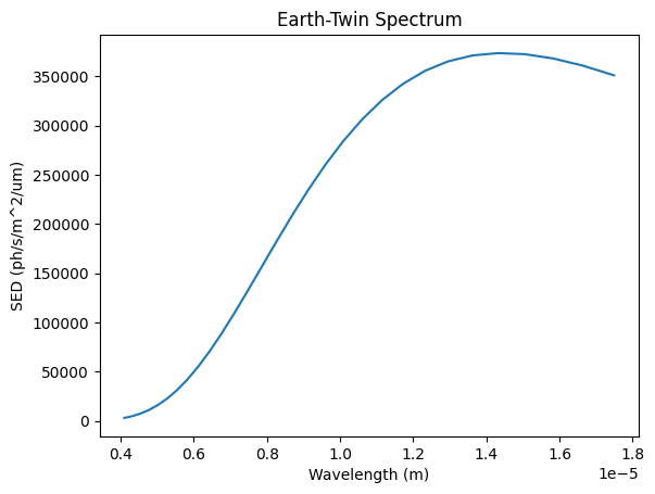
We can now also have a look at the spectra that have been generated for the sources:

earth_twin_spectrum = phringe.get_source_spectrum('Earth-Twin').cpu().numpy()[:, 0, 0]
wavelengths = phringe.get_wavelength_bin_centers().cpu().numpy()

plt.title('Earth-Twin Spectrum')
plt.plot(wavelengths, earth_twin_spectrum)
plt.ylabel('SED (ph/s/m^2/um)')
plt.xlabel('Wavelength (m)')
plt.show()

Once we have set an observation, an instrument and the star, we can also calculate the resulting nulling baseline length in meters (SI units):

phringe.get_nulling_baseline()

12.375888374825779

Run PHRINGE

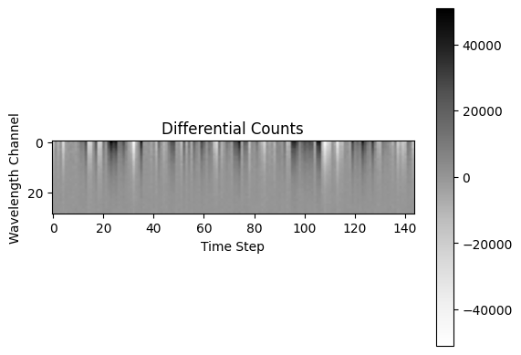
Calculate the Counts on the Detector

We calculate the raw counts at all four outputs of the nulling interferometer and use it to calculate the differential counts (on a CPU this is likely going to take a few tens of seconds).

counts = phringe.get_counts(kernels=True)

Plot the Differential Counts

Then we can plot the differential counts:

plt.imshow(counts.cpu().numpy()[0], cmap='Greys')
plt.title('Differential Counts')
plt.ylabel('Wavelength Channel')
plt.xlabel('Time Step')
plt.colorbar()
plt.show()

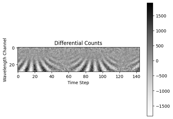
We now remove the instrument perturbations, increase the planet radius and reduce the radius of the star to see what impact this has on the data.

inst.amplitude_perturbation = None
inst.phase_perturbation = None
inst.polarization_perturbation = None
earth_twin.radius *= 2
sun_twin.radius /= 2

counts = phringe.get_counts(kernels=True)

As we can see, this not only reduces the counts on our detector, but also makes the planet signal appear. One could almost mistake this for the fur of a zebra…

plt.imshow(counts.cpu().numpy()[0], cmap='Greys')
plt.title('Differential Counts')
plt.ylabel('Wavelength Channel')
plt.xlabel('Time Step')
plt.colorbar()
plt.show()

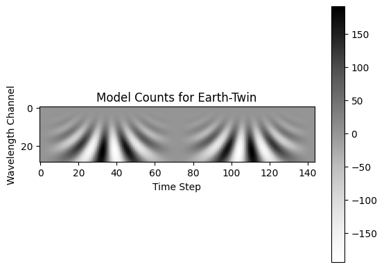
Compared to this, we can also have a look what the theoretical planet signal (template/model) would look like with a given spectrum and position:

model_counts = phringe.get_model_counts(
    kernels=True,
    spectral_energy_distribution=earth_twin_spectrum,
    x_position=3e-7,  # in radians
    y_position=0e-7  # in radians
)

plt.imshow(model_counts[0], cmap='Greys')
plt.title('Model Counts for Earth-Twin')
plt.ylabel('Wavelength Channel')
plt.xlabel('Time Step')
plt.colorbar()
plt.show()

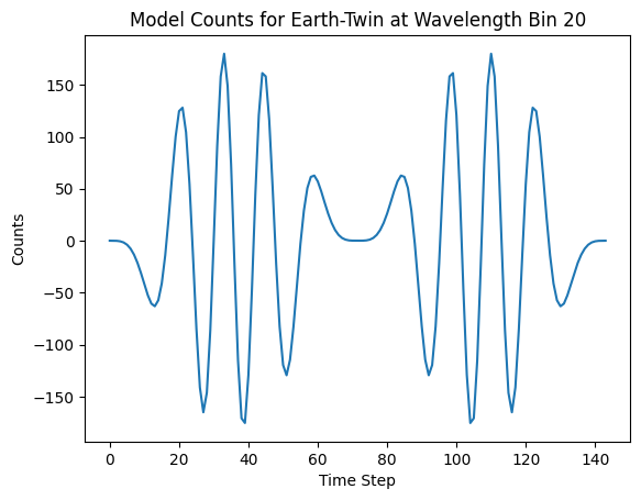
# Or at one wavelength
plt.plot(model_counts[0, 20])
plt.title('Model Counts for Earth-Twin at Wavelength Bin 20')
plt.ylabel('Counts')
plt.xlabel('Time Step')
plt.show()

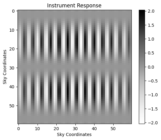
Plot Instrument Response

We can also have a look at the instrument response of our setup. To increase the resolution of this map increase the grid_size parameter when creating the PHRINGE object above.

fov_max = phringe.get_field_of_view()[0].item()
ir = phringe.get_instrument_response(fov=fov_max, kernels=True, perturbations=True)

# Get response at 10th wavelength bin and zeroth time step
ir = ir[:, 10, 0]

plt.imshow(ir.cpu().numpy()[0], cmap='Greys')
plt.title('Instrument Response')
plt.ylabel('Sky Coordinates')
plt.xlabel('Sky Coordinates')
plt.colorbar()
plt.show()

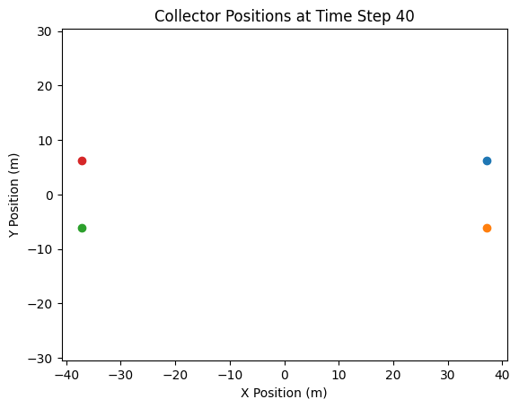
Plot Collector Positions

The collector positions can also be visualized easily:

col_pos = phringe.get_collector_positions()  # At time step 0

col_pos_x = col_pos[0]
col_pos_y = col_pos[1]

# Plot all four collectors at time step 0
for i in range(4):
    plt.scatter(col_pos_x[i, 0], col_pos_y[i, 0], label=f'Collector {i + 1}')
plt.title('Collector Positions at Time Step 40')
plt.xlabel('X Position (m)')
plt.ylabel('Y Position (m)')
plt.axis('equal')
plt.show()