Advanced Example

In this advanced example two input files, a spectrum file and a manually created Settings object are used to generate a basic data set for an Earth-like planet orbiting a Sun-like star 10 pc away. The Settings object will overwrite the settings specified in the config file. The code is run on GPU #0 in detailed mode, thus also saving and outputting the intensity responses.

Import modules and specify paths

from pathlib import Path

import matplotlib.pyplot as plt
import numpy as np
import torch

from phringe.api import PHRINGE
from phringe.core.entities.simulation import Simulation

config_file_path = Path('../_static/config.py')

Create Simulation Object

Note: passing a Simulation object to the run method will overwrite the simulation specified in the config file.

simulation = Simulation(
    grid_size=20,
    time_step_size='1 d',
    has_planet_orbital_motion=False,
    has_planet_signal=True,
    has_stellar_leakage=True,
    has_local_zodi_leakage=True,
    has_exozodi_leakage=True,
    has_amplitude_perturbations=True,
    has_phase_perturbations=True,
    has_polarization_perturbations=True
)

Run PHRINGE on GPU

Note the specification of the zeroth GPU to be used for the calculations. See the documentation of PHRINGE.run() for more information on the parameters.

phringe = PHRINGE()
phringe.run(
    config_file_path=config_file_path,
    simulation=simulation,
    gpu=0,
    fits_suffix='',
    write_fits=True,
    create_copy=True,
    normalize=False
)

Retrieve Basic Simulation Parameters

wavelengths = phringe.get_wavelength_bin_centers(as_numpy=True)
time_steps = phringe.get_time_steps(as_numpy=True)
fov = phringe.get_field_of_view(as_numpy=True)

Plot Data and Differential Intensity Response

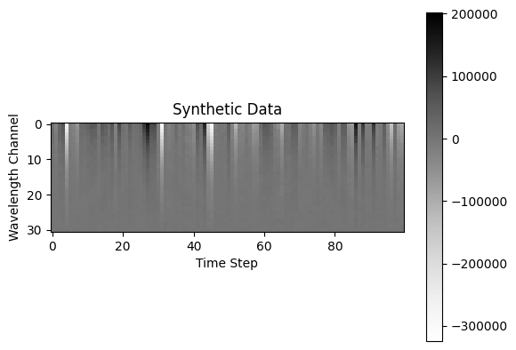
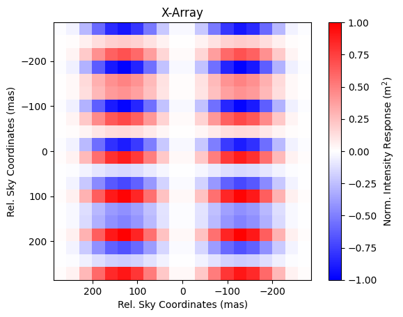
Plot the data in photoelectron counts and plot the corresponding (perturbed) differential intensity response.

data = phringe.get_data(as_numpy=True)
intensity_response = phringe.get_intensity_response_torch('Earth')
wavelengths = [round(wavelength * 1e6, 1) for wavelength in wavelengths]
time_steps = [int(round(time, 0)) for time in time_steps]
wavelength_index = 6
fov = (fov[wavelength_index] / 2) * 2.063e8
differential_ir = intensity_response[2, wavelength_index] - intensity_response[3, wavelength_index]
differential_ir /= torch.max(abs(differential_ir))

plt.imshow(data[0], cmap='Greys')
plt.title('Synthetic Data')
plt.ylabel('Wavelength Channel')
plt.xlabel('Time Step')
plt.colorbar()
plt.show()

im = plt.imshow(differential_ir[0], cmap='bwr', extent=(fov, -fov, fov, -fov), vmin=-1, vmax=1)
plt.title('X-Array')
plt.xlabel('Rel. Sky Coordinates (mas)')
plt.ylabel('Rel. Sky Coordinates (mas)')
cb = plt.colorbar(im)
cb.set_label(label='Norm. Intensity Response (m$^2$)')
plt.show()

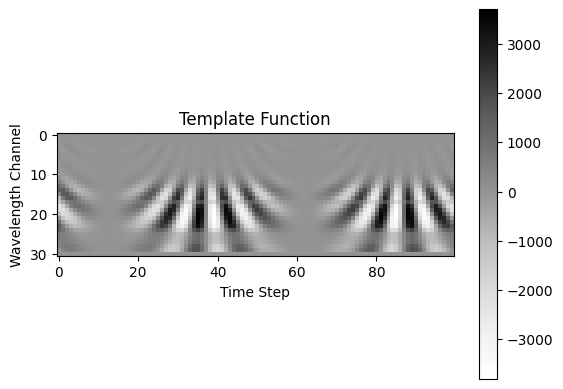
Plot the Template Function

Plot the template function corresponding to the (ideal, i.e. unperturbed) signal of a planet at a certain position in the field of view. Use the initial flux for the template generation.

time = phringe.get_time_steps(as_numpy=True)
wavelength_center = phringe.get_wavelength_bin_centers(as_numpy=True)
wavelength_bin = phringe.get_wavelength_bin_widths(as_numpy=True)
pos_x = np.array(3e-7)  # rad
pos_y = np.array(3e-7)  # rad
flux = phringe.get_spectral_flux_density('Earth', as_numpy=True)
template = phringe.get_template_numpy(time, wavelength_center, wavelength_bin, pos_x, pos_y, flux)

plt.imshow(template[0, :, :, 0, 0], cmap='Greys')
plt.title('Template Function')
plt.ylabel('Wavelength Channel')
plt.xlabel('Time Step')
plt.colorbar()
plt.show()